Statistical Functions
Percent Change
Series,DataFrame和Panel都有一个方法pct_change,用于计算给定时间段内的百分比变化(在之前使用fill_method填充NA / null值)。
In [1]: ser = pd.Series(np.random.randn(8))

In [2]: ser.pct_change()
Out[2]:
0         NaN
1   -1.602976
2    4.334938
3   -0.247456
4   -2.067345
5   -1.142903
6   -1.688214
7   -9.759729
dtype: float64
In [3]: df = pd.DataFrame(np.random.randn(10, 4))

In [4]: df.pct_change(periods=3)
Out[4]:
          0         1         2         3
0       NaN       NaN       NaN       NaN
1       NaN       NaN       NaN       NaN
2       NaN       NaN       NaN       NaN
3 -0.218320 -1.054001  1.987147 -0.510183
4 -0.439121 -1.816454  0.649715 -4.822809
5 -0.127833 -3.042065 -5.866604 -1.776977
6 -2.596833 -1.959538 -2.111697 -3.798900
7 -0.117826 -2.169058  0.036094 -0.067696
8  2.492606 -1.357320 -1.205802 -1.558697
9 -1.012977  2.324558 -1.003744 -0.371806
Covariance
Series对象具有方法cov以计算系列之间的协方差(不包括NA /空值)。
In [5]: s1 = pd.Series(np.random.randn(1000))

In [6]: s2 = pd.Series(np.random.randn(1000))

In [7]: s1.cov(s2)
Out[7]: 0.00068010881743108746
类似地,DataFrame具有方法cov以计算DataFrame中的系列之间的成对协方差,也不包括NA /空值。
注意
假设丢失的数据随机丢失,这导致对无偏差的协方差矩阵的估计。然而,对于许多应用,该估计可能是不可接受的,因为估计的协方差矩阵不能保证为正半定。这可以导致具有大于1的绝对值的估计相关,和/或不可逆协方差矩阵。有关详细信息,请参阅协方差矩阵估计。
In [8]: frame = pd.DataFrame(np.random.randn(1000, 5), columns=['a', 'b', 'c', 'd', 'e'])

In [9]: frame.cov()
Out[9]:
          a         b         c         d         e
a  1.000882 -0.003177 -0.002698 -0.006889  0.031912
b -0.003177  1.024721  0.000191  0.009212  0.000857
c -0.002698  0.000191  0.950735 -0.031743 -0.005087
d -0.006889  0.009212 -0.031743  1.002983 -0.047952
e  0.031912  0.000857 -0.005087 -0.047952  1.042487
DataFrame.cov还支持可选的min_periods关键字,该关键字指定每个列对所需的最小观测值数,以获得有效的结果。
In [10]: frame = pd.DataFrame(np.random.randn(20, 3), columns=['a', 'b', 'c'])

In [11]: frame.ix[:5, 'a'] = np.nan

In [12]: frame.ix[5:10, 'b'] = np.nan

In [13]: frame.cov()
Out[13]:
          a         b         c
a  1.210090 -0.430629  0.018002
b -0.430629  1.240960  0.347188
c  0.018002  0.347188  1.301149

In [14]: frame.cov(min_periods=12)
Out[14]:
          a         b         c
a  1.210090       NaN  0.018002
b       NaN  1.240960  0.347188
c  0.018002  0.347188  1.301149
Correlation
提供了用于计算相关性的几种方法:
| 方法名称 |
描述 |
|---|
pearson (默认) |
标准相关系数 |
kendall |
Kendall Tau相关系数 |
spearman |
斯皮尔曼等级相关系数 |
所有这些目前使用成对完全观察来计算。
In [15]: frame = pd.DataFrame(np.random.randn(1000, 5), columns=['a', 'b', 'c', 'd', 'e'])

In [16]: frame.ix[::2] = np.nan

# Series with Series
In [17]: frame['a'].corr(frame['b'])
Out[17]: 0.013479040400098775

In [18]: frame['a'].corr(frame['b'], method='spearman')
Out[18]: -0.0072898851595406371

# Pairwise correlation of DataFrame columns
In [19]: frame.corr()
Out[19]:
          a         b         c         d         e
a  1.000000  0.013479 -0.049269 -0.042239 -0.028525
b  0.013479  1.000000 -0.020433 -0.011139  0.005654
c -0.049269 -0.020433  1.000000  0.018587 -0.054269
d -0.042239 -0.011139  0.018587  1.000000 -0.017060
e -0.028525  0.005654 -0.054269 -0.017060  1.000000
请注意,非数字列将从相关性计算中自动排除。
像cov,corr也支持可选的min_periods关键字:
In [20]: frame = pd.DataFrame(np.random.randn(20, 3), columns=['a', 'b', 'c'])

In [21]: frame.ix[:5, 'a'] = np.nan

In [22]: frame.ix[5:10, 'b'] = np.nan

In [23]: frame.corr()
Out[23]:
          a         b         c
a  1.000000 -0.076520  0.160092
b -0.076520  1.000000  0.135967
c  0.160092  0.135967  1.000000

In [24]: frame.corr(min_periods=12)
Out[24]:
          a         b         c
a  1.000000       NaN  0.160092
b       NaN  1.000000  0.135967
c  0.160092  0.135967  1.000000
在DataFrame上实现相关方法corrwith,以计算不同DataFrame对象中包含的类似标记的系列之间的相关性。
In [25]: index = ['a', 'b', 'c', 'd', 'e']

In [26]: columns = ['one', 'two', 'three', 'four']

In [27]: df1 = pd.DataFrame(np.random.randn(5, 4), index=index, columns=columns)

In [28]: df2 = pd.DataFrame(np.random.randn(4, 4), index=index[:4], columns=columns)

In [29]: df1.corrwith(df2)
Out[29]:
one     -0.125501
two     -0.493244
three    0.344056
four     0.004183
dtype: float64

In [30]: df2.corrwith(df1, axis=1)
Out[30]:
a   -0.675817
b    0.458296
c    0.190809
d   -0.186275
e         NaN
dtype: float64
Data ranking
rank方法生成数据排名,其中系统分配了组的排名的平均值(默认情况下):
In [31]: s = pd.Series(np.random.np.random.randn(5), index=list('abcde'))

In [32]: s['d'] = s['b'] # so there's a tie

In [33]: s.rank()
Out[33]:
a    5.0
b    2.5
c    1.0
d    2.5
e    4.0
dtype: float64
rank也是DataFrame方法,可以对行(axis=0)或列(axis=1)排序。NaN值从排名中排除。
In [34]: df = pd.DataFrame(np.random.np.random.randn(10, 6))

In [35]: df[4] = df[2][:5] # some ties

In [36]: df
Out[36]:
          0         1         2         3         4         5
0 -0.904948 -1.163537 -1.457187  0.135463 -1.457187  0.294650
1 -0.976288 -0.244652 -0.748406 -0.999601 -0.748406 -0.800809
2  0.401965  1.460840  1.256057  1.308127  1.256057  0.876004
3  0.205954  0.369552 -0.669304  0.038378 -0.669304  1.140296
4 -0.477586 -0.730705 -1.129149 -0.601463 -1.129149 -0.211196
5 -1.092970 -0.689246  0.908114  0.204848       NaN  0.463347
6  0.376892  0.959292  0.095572 -0.593740       NaN -0.069180
7 -1.002601  1.957794 -0.120708  0.094214       NaN -1.467422
8 -0.547231  0.664402 -0.519424 -0.073254       NaN -1.263544
9 -0.250277 -0.237428 -1.056443  0.419477       NaN  1.375064

In [37]: df.rank(1)
Out[37]:
     0    1    2    3    4    5
0  4.0  3.0  1.5  5.0  1.5  6.0
1  2.0  6.0  4.5  1.0  4.5  3.0
2  1.0  6.0  3.5  5.0  3.5  2.0
3  4.0  5.0  1.5  3.0  1.5  6.0
4  5.0  3.0  1.5  4.0  1.5  6.0
5  1.0  2.0  5.0  3.0  NaN  4.0
6  4.0  5.0  3.0  1.0  NaN  2.0
7  2.0  5.0  3.0  4.0  NaN  1.0
8  2.0  5.0  3.0  4.0  NaN  1.0
9  2.0  3.0  1.0  4.0  NaN  5.0
rank可选地采用参数ascending,其默认为真;当为假时,数据被反向排序,其中较大的值被分配较小的等级。
rank支持使用method参数指定的不同的打破方法:
average:绑定组的平均排名min:组中的最低排名max:组中的最高排名first:按照它们在数组中显示的顺序分配的排名
Window Functions
警告
在版本0.18.0之前,pd.rolling_*,pd.expanding_*和pd.ewm*是模块级函数,现在已弃用。使用Rolling,Expanding和EWM替换这些。对象和相应的方法调用。
弃用警告将显示新语法,请参阅示例here您可以在此查看以前的文档
对于处理数据,提供了许多用于计算公共窗口或滚动 t>统计的窗口函数。其中包括计数,总和,平均值,中值,相关性,方差,协方差,标准偏差,偏度和峰度。
从版本0.18.1开始,可以直接从DataFrameGroupBy对象中使用rolling()和expanding()函数,请参阅groupby docs。
注意
窗口统计的API非常类似于使用GroupBy对象的方式,请参阅文档here
我们通过相应的对象处理rolling,expanding和指数式 加权 Rolling,Expanding和EWM。
In [38]: s = pd.Series(np.random.randn(1000), index=pd.date_range('1/1/2000', periods=1000))

In [39]: s = s.cumsum()

In [40]: s
Out[40]:
2000-01-01    -0.268824
2000-01-02    -1.771855
2000-01-03    -0.818003
2000-01-04    -0.659244
2000-01-05    -1.942133
2000-01-06    -1.869391
2000-01-07     0.563674
                ...
2002-09-20   -68.233054
2002-09-21   -66.765687
2002-09-22   -67.457323
2002-09-23   -69.253182
2002-09-24   -70.296818
2002-09-25   -70.844674
2002-09-26   -72.475016
Freq: D, dtype: float64
这些是从Series和DataFrame的方法创建的。
In [41]: r = s.rolling(window=60)

In [42]: r
Out[42]: Rolling [window=60,center=False,axis=0]
这些对象提供了可选方法和属性的制表完成。
In [14]: r.
r.agg         r.apply       r.count       r.exclusions  r.max         r.median      r.name        r.skew        r.sum
r.aggregate   r.corr        r.cov         r.kurt        r.mean        r.min         r.quantile    r.std         r.var
通常这些方法都有相同的接口。他们都接受以下参数:
window:移动窗口的大小min_periods:要求非空数据点的阈值(否则结果为NA)center:boolean,是否将标签设置在中心(默认为False)
警告
在0.18.0更改之前,freq和how参数在API中。这些在新的API中已弃用。您可以在创建窗口函数之前对输入进行简单重新采样。
例如,代替s.rolling(window=5,freq='D').max()在滚动5天窗口中获取最大值,可以使用s.resample('D').max().rolling(window=5).max(),首先将数据重新采样为每日数据,然后提供滚动5天窗口。
然后,我们可以在这些rolling对象上调用方法。这些返回类似索引的对象:
In [43]: r.mean()
Out[43]:
2000-01-01          NaN
2000-01-02          NaN
2000-01-03          NaN
2000-01-04          NaN
2000-01-05          NaN
2000-01-06          NaN
2000-01-07          NaN
                ...
2002-09-20   -62.694135
2002-09-21   -62.812190
2002-09-22   -62.914971
2002-09-23   -63.061867
2002-09-24   -63.213876
2002-09-25   -63.375074
2002-09-26   -63.539734
Freq: D, dtype: float64
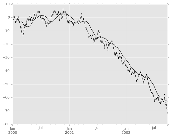
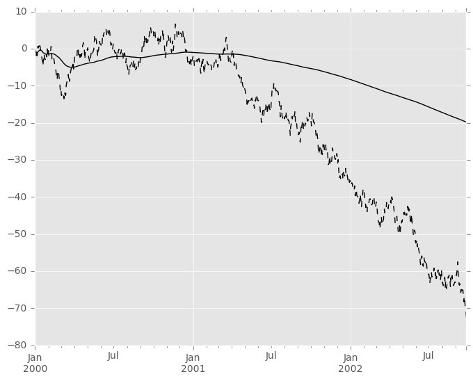
In [44]: s.plot(style='k--')
Out[44]: <matplotlib.axes._subplots.AxesSubplot at 0x7ff282080dd0>

In [45]: r.mean().plot(style='k')
Out[45]: <matplotlib.axes._subplots.AxesSubplot at 0x7ff282080dd0>
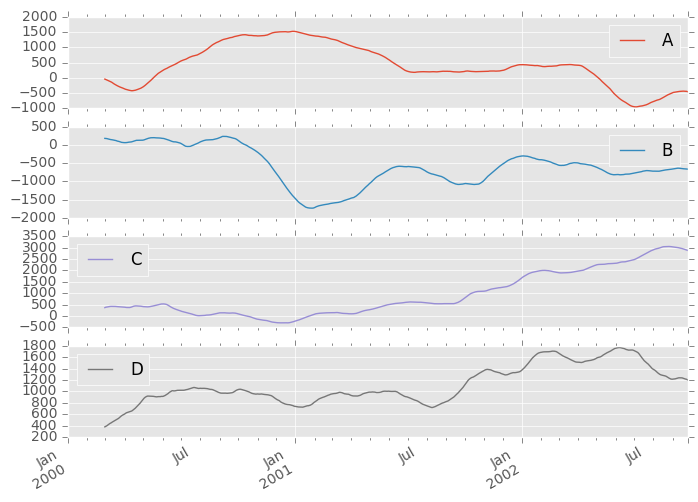
它们也可以应用于DataFrame对象。这实际上只是语法糖用于移动窗口运算符到所有的DataFrame的列:
In [46]: df = pd.DataFrame(np.random.randn(1000, 4),
   ....:                   index=pd.date_range('1/1/2000', periods=1000),
   ....:                   columns=['A', 'B', 'C', 'D'])
   ....:

In [47]: df = df.cumsum()

In [48]: df.rolling(window=60).sum().plot(subplots=True)
Out[48]:
array([<matplotlib.axes._subplots.AxesSubplot object at 0x7ff28c067210>,
       <matplotlib.axes._subplots.AxesSubplot object at 0x7ff27e03a0d0>,
       <matplotlib.axes._subplots.AxesSubplot object at 0x7ff280bca510>,
       <matplotlib.axes._subplots.AxesSubplot object at 0x7ff28155b910>], dtype=object)
Method Summary
我们提供了一些常见的统计功能:
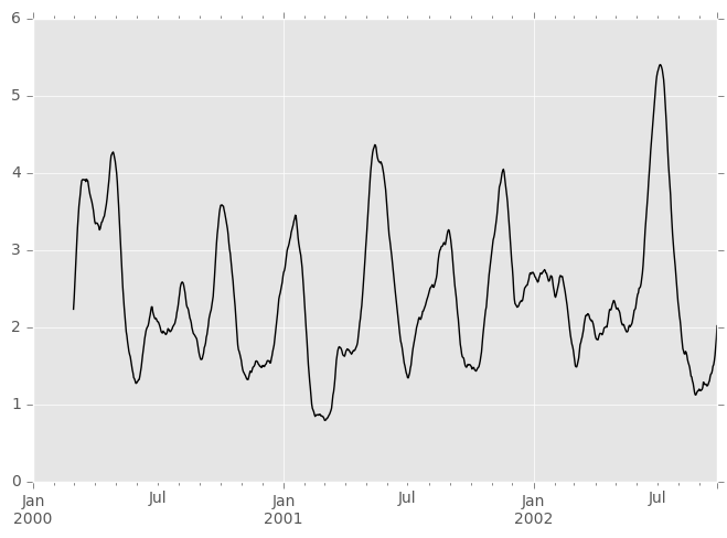
apply()函数需要一个额外的func参数,并执行通用滚动计算。func参数应该是一个从ndarray输入生成单个值的单个函数。假设我们想要计算滚动平均绝对偏差:
In [49]: mad = lambda x: np.fabs(x - x.mean()).mean()

In [50]: s.rolling(window=60).apply(mad).plot(style='k')
Out[50]: <matplotlib.axes._subplots.AxesSubplot at 0x7ff2846d3ad0>
Rolling Windows
将win_type传递到.rolling生成通用滚动窗口计算,根据win_type进行加权。提供以下方法:
窗口中使用的权重由win_type关键字指定。公认类型的列表是:
boxcartriangblackmanhammingbartlettparzenbohmanblackmanharrisnuttallbarthannkaiser(需要测试版)gaussian(needs std)general_gaussian(需要功率,宽度)slepian(需要宽度)。
In [51]: ser = pd.Series(np.random.randn(10), index=pd.date_range('1/1/2000', periods=10))

In [52]: ser.rolling(window=5, win_type='triang').mean()
Out[52]:
2000-01-01         NaN
2000-01-02         NaN
2000-01-03         NaN
2000-01-04         NaN
2000-01-05   -1.037870
2000-01-06   -0.767705
2000-01-07   -0.383197
2000-01-08   -0.395513
2000-01-09   -0.558440
2000-01-10   -0.672416
Freq: D, dtype: float64
注意,boxcar窗口等效于mean()。
In [53]: ser.rolling(window=5, win_type='boxcar').mean()
Out[53]:
2000-01-01         NaN
2000-01-02         NaN
2000-01-03         NaN
2000-01-04         NaN
2000-01-05   -0.841164
2000-01-06   -0.779948
2000-01-07   -0.565487
2000-01-08   -0.502815
2000-01-09   -0.553755
2000-01-10   -0.472211
Freq: D, dtype: float64

In [54]: ser.rolling(window=5).mean()
Out[54]:
2000-01-01         NaN
2000-01-02         NaN
2000-01-03         NaN
2000-01-04         NaN
2000-01-05   -0.841164
2000-01-06   -0.779948
2000-01-07   -0.565487
2000-01-08   -0.502815
2000-01-09   -0.553755
2000-01-10   -0.472211
Freq: D, dtype: float64
对于某些窗口函数,必须指定其他参数:
In [55]: ser.rolling(window=5, win_type='gaussian').mean(std=0.1)
Out[55]:
2000-01-01         NaN
2000-01-02         NaN
2000-01-03         NaN
2000-01-04         NaN
2000-01-05   -1.309989
2000-01-06   -1.153000
2000-01-07    0.606382
2000-01-08   -0.681101
2000-01-09   -0.289724
2000-01-10   -0.996632
Freq: D, dtype: float64
注意
对于具有win_type的.sum(),对于窗口的权重没有进行归一化。传递[1, 1, 1]的自定义权重将产生与传递 [2, 2, 2]。当传递win_type而不是显式地指定权重时,权重已经被归一化,使得最大权重为1。
相反,.mean()计算的性质使得权重相对于彼此被标准化。[1, 1, 1]和[2, t5 > 2, 2]产生相同的结果。
Time-aware Rolling
版本0.19.0中的新功能是将偏移量(或可转换)传递给.rolling()方法,并根据传递的时间窗口生成可变大小的窗口。对于每个时间点,这包括在指示的时间Δ内出现的所有先前值。
这对于非规则的时间频率指数特别有用。
In [56]: dft = pd.DataFrame({'B': [0, 1, 2, np.nan, 4]},
   ....:                    index=pd.date_range('20130101 09:00:00', periods=5, freq='s'))
   ....:

In [57]: dft
Out[57]:
                       B
2013-01-01 09:00:00  0.0
2013-01-01 09:00:01  1.0
2013-01-01 09:00:02  2.0
2013-01-01 09:00:03  NaN
2013-01-01 09:00:04  4.0
这是一个常规的频率指数。使用整数窗口参数可以沿窗口频率滚动。
In [58]: dft.rolling(2).sum()
Out[58]:
                       B
2013-01-01 09:00:00  NaN
2013-01-01 09:00:01  1.0
2013-01-01 09:00:02  3.0
2013-01-01 09:00:03  NaN
2013-01-01 09:00:04  NaN

In [59]: dft.rolling(2, min_periods=1).sum()
Out[59]:
                       B
2013-01-01 09:00:00  0.0
2013-01-01 09:00:01  1.0
2013-01-01 09:00:02  3.0
2013-01-01 09:00:03  2.0
2013-01-01 09:00:04  4.0
指定偏移允许更直观地规定滚动频率。
In [60]: dft.rolling('2s').sum()
Out[60]:
                       B
2013-01-01 09:00:00  0.0
2013-01-01 09:00:01  1.0
2013-01-01 09:00:02  3.0
2013-01-01 09:00:03  2.0
2013-01-01 09:00:04  4.0
使用非规则但仍然是单调的索引,使用整数窗口滚动不会赋予任何特殊的计算。
In [61]: dft = pd.DataFrame({'B': [0, 1, 2, np.nan, 4]},
   ....:                    index = pd.Index([pd.Timestamp('20130101 09:00:00'),
   ....:                                      pd.Timestamp('20130101 09:00:02'),
   ....:                                      pd.Timestamp('20130101 09:00:03'),
   ....:                                      pd.Timestamp('20130101 09:00:05'),
   ....:                                      pd.Timestamp('20130101 09:00:06')],
   ....:                                     name='foo'))
   ....:

In [62]: dft
Out[62]:
                       B
foo
2013-01-01 09:00:00  0.0
2013-01-01 09:00:02  1.0
2013-01-01 09:00:03  2.0
2013-01-01 09:00:05  NaN
2013-01-01 09:00:06  4.0

In [63]: dft.rolling(2).sum()
Out[63]:
                       B
foo
2013-01-01 09:00:00  NaN
2013-01-01 09:00:02  1.0
2013-01-01 09:00:03  3.0
2013-01-01 09:00:05  NaN
2013-01-01 09:00:06  NaN
使用时间规范为这个稀疏数据生成变量窗口。
In [64]: dft.rolling('2s').sum()
Out[64]:
                       B
foo
2013-01-01 09:00:00  0.0
2013-01-01 09:00:02  1.0
2013-01-01 09:00:03  3.0
2013-01-01 09:00:05  NaN
2013-01-01 09:00:06  4.0
此外,我们现在允许一个可选的on参数在DataFrame中指定一个列(而不是索引的默认值)。
In [65]: dft = dft.reset_index()

In [66]: dft
Out[66]:
                  foo    B
0 2013-01-01 09:00:00  0.0
1 2013-01-01 09:00:02  1.0
2 2013-01-01 09:00:03  2.0
3 2013-01-01 09:00:05  NaN
4 2013-01-01 09:00:06  4.0

In [67]: dft.rolling('2s', on='foo').sum()
Out[67]:
                  foo    B
0 2013-01-01 09:00:00  0.0
1 2013-01-01 09:00:02  1.0
2 2013-01-01 09:00:03  3.0
3 2013-01-01 09:00:05  NaN
4 2013-01-01 09:00:06  4.0
Time-aware Rolling vs. Resampling
使用.rolling()与基于时间的索引非常类似于resampling。它们都对时间索引的pandas对象进行操作和执行还原操作。
当使用带偏移的.rolling()时。偏移量是时间增量。采取后向时间窗口,并聚合该窗口中的所有值(包括端点,但不是开始点)。这是在结果中的那个点的新值。这些是在输入的每个点的时间空间中的可变大小的窗口。您将获得与输入相同大小的结果。
当使用带偏移量的.resample()时。构造一个新的索引,即偏移的频率。对于每个频率仓,在落入该仓中的向后时间查看窗口内的来自输入的聚合点。此聚合的结果是该频点的输出。窗口在频率空间中是固定大小尺寸。您的结果将具有在原始输入对象的最小值和最大值之间的常规频率的形状。
总而言之,.rolling()是基于时间的窗口操作,而.resample()是基于频率的窗口操作。
Centering Windows
默认情况下,标签设置为窗口的右边缘,但是可以使用center关键字,因此可以将标签设置在中心。
In [68]: ser.rolling(window=5).mean()
Out[68]:
2000-01-01         NaN
2000-01-02         NaN
2000-01-03         NaN
2000-01-04         NaN
2000-01-05   -0.841164
2000-01-06   -0.779948
2000-01-07   -0.565487
2000-01-08   -0.502815
2000-01-09   -0.553755
2000-01-10   -0.472211
Freq: D, dtype: float64

In [69]: ser.rolling(window=5, center=True).mean()
Out[69]:
2000-01-01         NaN
2000-01-02         NaN
2000-01-03   -0.841164
2000-01-04   -0.779948
2000-01-05   -0.565487
2000-01-06   -0.502815
2000-01-07   -0.553755
2000-01-08   -0.472211
2000-01-09         NaN
2000-01-10         NaN
Freq: D, dtype: float64
Binary Window Functions
cov()和corr()可以计算关于两个Series或DataFrame/Series或DataFrame/DataFrame。这里是每种情况下的行为:
- 两个
Series:计算配对的统计信息。
DataFrame/Series:使用传递的Series计算DataFrame的每个列的统计信息,从而返回一个DataFrame。DataFrame/DataFrame:默认情况下计算匹配列名称的统计信息,返回DataFrame。如果传递关键字参数pairwise=True,则计算每对列的统计量,返回Panel,其items (见the next section)。
例如:
In [70]: df2 = df[:20]

In [71]: df2.rolling(window=5).corr(df2['B'])
Out[71]:
                   A    B         C         D
2000-01-01       NaN  NaN       NaN       NaN
2000-01-02       NaN  NaN       NaN       NaN
2000-01-03       NaN  NaN       NaN       NaN
2000-01-04       NaN  NaN       NaN       NaN
2000-01-05 -0.262853  1.0  0.334449  0.193380
2000-01-06 -0.083745  1.0 -0.521587 -0.556126
2000-01-07 -0.292940  1.0 -0.658532 -0.458128
...              ...  ...       ...       ...
2000-01-14  0.519499  1.0 -0.687277  0.192822
2000-01-15  0.048982  1.0  0.167669 -0.061463
2000-01-16  0.217190  1.0  0.167564 -0.326034
2000-01-17  0.641180  1.0 -0.164780 -0.111487
2000-01-18  0.130422  1.0  0.322833  0.632383
2000-01-19  0.317278  1.0  0.384528  0.813656
2000-01-20  0.293598  1.0  0.159538  0.742381

[20 rows x 4 columns]
Computing rolling pairwise covariances and correlations
在金融数据分析和其他领域中,通常对于时间序列的集合计算协方差和相关矩阵。通常,人们也对移动窗协方差和相关矩阵感兴趣。This can be done by passing the pairwise keyword argument, which in the case of DataFrame inputs will yield a Panel whose items are the dates in question. 在单个DataFrame参数的情况下,甚至可以省略pairwise参数:
In [72]: covs = df[['B','C','D']].rolling(window=50).cov(df[['A','B','C']], pairwise=True)

In [73]: covs[df.index[-50]]
Out[73]:
          A         B          C
B  2.667506  1.671711   1.938634
C  8.513843  1.938634  10.556436
D -7.714737 -1.434529  -7.082653
In [74]: correls = df.rolling(window=50).corr()

In [75]: correls[df.index[-50]]
Out[75]:
          A         B         C         D
A  1.000000  0.604221  0.767429 -0.776170
B  0.604221  1.000000  0.461484 -0.381148
C  0.767429  0.461484  1.000000 -0.748863
D -0.776170 -0.381148 -0.748863  1.000000
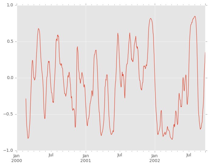
您可以使用.loc索引有效地检索两列之间的相关性的时间序列:
In [76]: correls.loc[:, 'A', 'C'].plot()
Out[76]: <matplotlib.axes._subplots.AxesSubplot at 0x7ff27e0f0c50>
Aggregation
一旦创建了Rolling,Expanding或EWM对象,就有几种方法可以对数据执行多个计算。这非常类似于.groupby(...).agg看到here。
In [77]: dfa = pd.DataFrame(np.random.randn(1000, 3),
   ....:                    index=pd.date_range('1/1/2000', periods=1000),
   ....:                    columns=['A', 'B', 'C'])
   ....:

In [78]: r = dfa.rolling(window=60,min_periods=1)

In [79]: r
Out[79]: Rolling [window=60,min_periods=1,center=False,axis=0]
我们可以通过传递一个函数到整个DataFrame,或通过标准的getitem选择一个系列(或多个系列)。
In [80]: r.aggregate(np.sum)
Out[80]:
                   A          B         C
2000-01-01  0.314226  -0.001675  0.071823
2000-01-02  1.206791   0.678918 -0.267817
2000-01-03  1.421701   0.600508 -0.445482
2000-01-04  1.912539  -0.759594  1.146974
2000-01-05  2.919639  -0.061759 -0.743617
2000-01-06  2.665637   1.298392 -0.803529
2000-01-07  2.513985   1.923089 -1.928308
...              ...        ...       ...
2002-09-20  1.447669 -12.360302  2.734381
2002-09-21  1.871783 -13.896542  3.086102
2002-09-22  2.540658 -12.594402  3.162542
2002-09-23  2.974674 -12.727703  3.861005
2002-09-24  1.391366 -13.584590  3.790683
2002-09-25  2.027313 -15.083214  3.377896
2002-09-26  1.290363 -13.569459  3.809884

[1000 rows x 3 columns]

In [81]: r['A'].aggregate(np.sum)
Out[81]:
2000-01-01    0.314226
2000-01-02    1.206791
2000-01-03    1.421701
2000-01-04    1.912539
2000-01-05    2.919639
2000-01-06    2.665637
2000-01-07    2.513985
                ...
2002-09-20    1.447669
2002-09-21    1.871783
2002-09-22    2.540658
2002-09-23    2.974674
2002-09-24    1.391366
2002-09-25    2.027313
2002-09-26    1.290363
Freq: D, Name: A, dtype: float64

In [82]: r[['A','B']].aggregate(np.sum)
Out[82]:
                   A          B
2000-01-01  0.314226  -0.001675
2000-01-02  1.206791   0.678918
2000-01-03  1.421701   0.600508
2000-01-04  1.912539  -0.759594
2000-01-05  2.919639  -0.061759
2000-01-06  2.665637   1.298392
2000-01-07  2.513985   1.923089
...              ...        ...
2002-09-20  1.447669 -12.360302
2002-09-21  1.871783 -13.896542
2002-09-22  2.540658 -12.594402
2002-09-23  2.974674 -12.727703
2002-09-24  1.391366 -13.584590
2002-09-25  2.027313 -15.083214
2002-09-26  1.290363 -13.569459

[1000 rows x 2 columns]
正如您所看到的,聚合的结果将包含所选列,或者如果没有选择列,则包含所有列。
Applying multiple functions at once
使用windowed系列,您还可以传递函数的列表或字典以进行聚合,输出DataFrame:
In [83]: r['A'].agg([np.sum, np.mean, np.std])
Out[83]:
                 sum      mean       std
2000-01-01  0.314226  0.314226       NaN
2000-01-02  1.206791  0.603396  0.408948
2000-01-03  1.421701  0.473900  0.365959
2000-01-04  1.912539  0.478135  0.298925
2000-01-05  2.919639  0.583928  0.350682
2000-01-06  2.665637  0.444273  0.464115
2000-01-07  2.513985  0.359141  0.479828
...              ...       ...       ...
2002-09-20  1.447669  0.024128  1.034827
2002-09-21  1.871783  0.031196  1.031417
2002-09-22  2.540658  0.042344  1.026341
2002-09-23  2.974674  0.049578  1.030021
2002-09-24  1.391366  0.023189  1.024793
2002-09-25  2.027313  0.033789  1.022099
2002-09-26  1.290363  0.021506  1.024751

[1000 rows x 3 columns]
如果传递了dict,则键将用于命名列。否则将使用函数的名称(存储在函数对象中)。
In [84]: r['A'].agg({'result1' : np.sum,
   ....:             'result2' : np.mean})
   ....:
Out[84]:
             result2   result1
2000-01-01  0.314226  0.314226
2000-01-02  0.603396  1.206791
2000-01-03  0.473900  1.421701
2000-01-04  0.478135  1.912539
2000-01-05  0.583928  2.919639
2000-01-06  0.444273  2.665637
2000-01-07  0.359141  2.513985
...              ...       ...
2002-09-20  0.024128  1.447669
2002-09-21  0.031196  1.871783
2002-09-22  0.042344  2.540658
2002-09-23  0.049578  2.974674
2002-09-24  0.023189  1.391366
2002-09-25  0.033789  2.027313
2002-09-26  0.021506  1.290363

[1000 rows x 2 columns]
在寡居式DataFrame上,您可以传递要应用于每个列的函数列表,这将生成带有层次索引的聚合结果:
In [85]: r.agg([np.sum, np.mean])
Out[85]:
                   A                    B                   C
                 sum      mean        sum      mean       sum      mean
2000-01-01  0.314226  0.314226  -0.001675 -0.001675  0.071823  0.071823
2000-01-02  1.206791  0.603396   0.678918  0.339459 -0.267817 -0.133908
2000-01-03  1.421701  0.473900   0.600508  0.200169 -0.445482 -0.148494
2000-01-04  1.912539  0.478135  -0.759594 -0.189899  1.146974  0.286744
2000-01-05  2.919639  0.583928  -0.061759 -0.012352 -0.743617 -0.148723
2000-01-06  2.665637  0.444273   1.298392  0.216399 -0.803529 -0.133921
2000-01-07  2.513985  0.359141   1.923089  0.274727 -1.928308 -0.275473
...              ...       ...        ...       ...       ...       ...
2002-09-20  1.447669  0.024128 -12.360302 -0.206005  2.734381  0.045573
2002-09-21  1.871783  0.031196 -13.896542 -0.231609  3.086102  0.051435
2002-09-22  2.540658  0.042344 -12.594402 -0.209907  3.162542  0.052709
2002-09-23  2.974674  0.049578 -12.727703 -0.212128  3.861005  0.064350
2002-09-24  1.391366  0.023189 -13.584590 -0.226410  3.790683  0.063178
2002-09-25  2.027313  0.033789 -15.083214 -0.251387  3.377896  0.056298
2002-09-26  1.290363  0.021506 -13.569459 -0.226158  3.809884  0.063498

[1000 rows x 6 columns]
默认情况下,传递函数的dict具有不同的行为,请参见下一节。
Applying different functions to DataFrame columns
通过将dict传递到aggregate,您可以对DataFrame的列应用不同的聚合:
In [86]: r.agg({'A' : np.sum,
   ....:        'B' : lambda x: np.std(x, ddof=1)})
   ....:
Out[86]:
                   A         B
2000-01-01  0.314226       NaN
2000-01-02  1.206791  0.482437
2000-01-03  1.421701  0.417825
2000-01-04  1.912539  0.851468
2000-01-05  2.919639  0.837474
2000-01-06  2.665637  0.935441
2000-01-07  2.513985  0.867770
...              ...       ...
2002-09-20  1.447669  1.084259
2002-09-21  1.871783  1.088368
2002-09-22  2.540658  1.084707
2002-09-23  2.974674  1.084936
2002-09-24  1.391366  1.079268
2002-09-25  2.027313  1.091334
2002-09-26  1.290363  1.060255

[1000 rows x 2 columns]
函数名也可以是字符串。为了使字符串有效,它必须在窗口对象上实现
In [87]: r.agg({'A' : 'sum', 'B' : 'std'})
Out[87]:
                   A         B
2000-01-01  0.314226       NaN
2000-01-02  1.206791  0.482437
2000-01-03  1.421701  0.417825
2000-01-04  1.912539  0.851468
2000-01-05  2.919639  0.837474
2000-01-06  2.665637  0.935441
2000-01-07  2.513985  0.867770
...              ...       ...
2002-09-20  1.447669  1.084259
2002-09-21  1.871783  1.088368
2002-09-22  2.540658  1.084707
2002-09-23  2.974674  1.084936
2002-09-24  1.391366  1.079268
2002-09-25  2.027313  1.091334
2002-09-26  1.290363  1.060255

[1000 rows x 2 columns]
此外,您可以传递嵌套dict以指示不同列上的不同聚合。
In [88]: r.agg({'A' : ['sum','std'], 'B' : ['mean','std'] })
Out[88]:
                   A                   B
                 sum       std      mean       std
2000-01-01  0.314226       NaN -0.001675       NaN
2000-01-02  1.206791  0.408948  0.339459  0.482437
2000-01-03  1.421701  0.365959  0.200169  0.417825
2000-01-04  1.912539  0.298925 -0.189899  0.851468
2000-01-05  2.919639  0.350682 -0.012352  0.837474
2000-01-06  2.665637  0.464115  0.216399  0.935441
2000-01-07  2.513985  0.479828  0.274727  0.867770
...              ...       ...       ...       ...
2002-09-20  1.447669  1.034827 -0.206005  1.084259
2002-09-21  1.871783  1.031417 -0.231609  1.088368
2002-09-22  2.540658  1.026341 -0.209907  1.084707
2002-09-23  2.974674  1.030021 -0.212128  1.084936
2002-09-24  1.391366  1.024793 -0.226410  1.079268
2002-09-25  2.027313  1.022099 -0.251387  1.091334
2002-09-26  1.290363  1.024751 -0.226158  1.060255

[1000 rows x 4 columns]
Expanding Windows
滚动统计的一个常见替代方法是使用展开窗口,该窗口会生成带有在该时间点之前可用的所有数据的统计值。
这些跟随类似的.rolling界面,.expanding方法返回一个Expanding对象。
因为这些计算是滚动统计的特殊情况,所以它们在pandas中实现,使得以下两个调用是等效的:
In [89]: df.rolling(window=len(df), min_periods=1).mean()[:5]
Out[89]:
                   A         B         C         D
2000-01-01 -1.388345  3.317290  0.344542 -0.036968
2000-01-02 -1.123132  3.622300  1.675867  0.595300
2000-01-03 -0.628502  3.626503  2.455240  1.060158
2000-01-04 -0.768740  3.888917  2.451354  1.281874
2000-01-05 -0.824034  4.108035  2.556112  1.140723

In [90]: df.expanding(min_periods=1).mean()[:5]
Out[90]:
                   A         B         C         D
2000-01-01 -1.388345  3.317290  0.344542 -0.036968
2000-01-02 -1.123132  3.622300  1.675867  0.595300
2000-01-03 -0.628502  3.626503  2.455240  1.060158
2000-01-04 -0.768740  3.888917  2.451354  1.281874
2000-01-05 -0.824034  4.108035  2.556112  1.140723
这些方法具有与.rolling方法类似的一组方法。
Method Summary
除了不具有window参数,这些函数具有与它们的.rolling对等体相同的接口。像上面一样,它们都接受的参数是:
min_periods:要求的非空数据点的阈值。默认为计算统计所需的最小值。在看到min_periods非空数据点后,将不输出NaNs。center:boolean,是否将标签设置在中心(默认为False)
注意
.rolling和.expanding方法的输出不返回NaN,如果至少有min_periods - 当前窗口中的空值。This differs from cumsum, cumprod, cummax, and cummin, which return NaN in the output wherever a NaN is encountered in the input.
扩展窗口统计将比其滚动窗口对应更稳定(并且响应更少),因为增加的窗口大小减小了单个数据点的相对影响。例如,以下是上一个时间序列数据集的mean()输出:
In [91]: s.plot(style='k--')
Out[91]: <matplotlib.axes._subplots.AxesSubplot at 0x7ff29c7378d0>

In [92]: s.expanding().mean().plot(style='k')
Out[92]: <matplotlib.axes._subplots.AxesSubplot at 0x7ff29c7378d0>
Exponentially Weighted Windows
相关的一组函数是几个上述统计量的指数加权版本。通过.ewm方法访问与.rolling和.expanding类似的接口,以接收EWM对象。提供了许多扩展EW(指数加权)方法:
一般来说,加权移动平均值计算为
y_t = \ frac {\ sum_ {i = 0} ^ t w_i x_ {t-i}} {\ sum_ {i = 0} ^ t w_i},
其中x_t是输入,y_t是结果。
EW函数支持指数权重的两种变体。默认值adjust=True使用权重w_i =(1 - \ alpha)^ i
y_t = \ frac {x_t +(1-αalpha)x_ {t-1} +(1-αalpha)^ 2 x_ {t-2} + ... + x_ {0}} {1 +(1-αα)+(1-αα)^ 2 + ... +(1-αα)
当指定adjust=False时,移动平均值计算为
y_0&amp; = x_0 \\ y_t&amp; =(1 - \ alpha)y_ {t-1} + \ alpha x_t,
这相当于使用权重
w_i = \ begin {cases} \ alpha(1 - \ alpha)^ i&amp; \ text {if} i
注意
这些方程有时用\ alpha'= 1-\α来表示,例如。
y_t = \ alpha'y_ {t-1} +(1 - \ alpha')x_t。
上述两种变体之间的区别出现是因为我们处理具有有限历史的系列。考虑一系列无限历史:
y_t = \ frac {x_t +(1-αalpha)x_ {t-1} +(1-αalpha)^ 2 x_ {t-2} + ...} {1 +(1 - \ alpha )+(1-αα)^ 2 + ...}
注意到分母是几何级数,其初始项等于1,比率为1 - \ alpha
y_t&amp; = \ frac {x_t +(1 - \ alpha)x_ {t-1} +(1 - \ alpha)^ 2 x_ {t-2} + ...} {\ frac {1} {1-(1-α)}} \\&amp; = [x_t +(1-α)x_ {t-1} +(1-αα)^ 2 x_ {t-2} + ... ] \ alpha \\&amp; = \ alpha x_t + [(1- \ alpha)x_ {t-1} +(1-\ alpha)^ 2 x_ {t-2} + ...] \ alpha \\&amp; ; = \ alpha x_t +(1 - \ alpha)[x_ {t-1} +(1 - \ alpha)x_ {t-2} + ...] \ alpha \\&amp; = \ alpha x_t + - \ alpha)y_ {t-1}
其示出了上述两个变量对于无穷级数的等价。当adjust=True时,我们有y_0 = x_0,从上面的最后一个表示中,我们有y_t = \ alpha x_t +(1 - \ alpha)y_ { 1},因此假设x_0不是普通值,而是直到该点的无限序列的指数加权矩。
必须有0 ,而自版本0.18.0以来,可以直接传递\ alpha,通常更容易考虑span ,质心(com)或半衰期
\ alpha = \ begin {cases} \ frac {2} {s + 1},&amp; \ text {for span} \ s \ geq 1 \\ \ frac {1} {1 + c},&amp; \ text {for center of mass} \ c \ geq 0 \\ 1 - \ exp ^ {\ frac {\ log 0.5} {h}},&amp; \ text {for half-life} \ h&gt; 0 \ end {cases}
必须精确地指定EW功能的span,质心,半衰期和
- 跨度对应于通常所称的“N日EW移动平均线”。
- 质心具有更多的物理解释,可以在跨度方面考虑:c =(s-1)/ 2。
- 半衰期是指数权重减少到一半的时间段。
- Alpha直接指定平滑因子。
以下是单变量时间序列的示例:
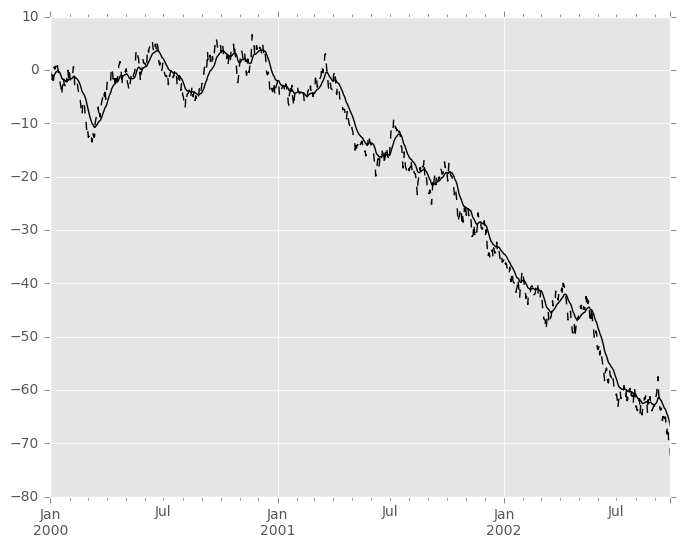
In [93]: s.plot(style='k--')
Out[93]: <matplotlib.axes._subplots.AxesSubplot at 0x7ff29c73bdd0>

In [94]: s.ewm(span=20).mean().plot(style='k')
Out[94]: <matplotlib.axes._subplots.AxesSubplot at 0x7ff29c73bdd0>
EWM有一个min_periods参数,它具有与所有.expanding和.rolling方法相同的含义:将不设置输出值直到在(扩展)窗口中遇到至少min_periods个非空值。(这是从0.15.0之前的版本的变化,其中min_periods参数仅影响从第一个非空值开始的min_periods连续条目。)
EWM还有一个ignore_na参数,它决定了中间空值如何影响权重的计算。当ignore_na=False(默认值)时,将根据绝对位置计算权重,以使中间空值影响结果。当ignore_na=True(重现0.15.0之前的版本中的行为)时,通过忽略中间空值计算权重。For example, assuming adjust=True, if ignore_na=False, the weighted average of 3, NaN, 5 would be calculated as
\ frac {(1- \ alpha)^ 2 \ cdot 3 + 1 \ cdot 5} {(1 \ alpha)^ 2 + 1}
而如果ignore_na=True,加权平均值将被计算为
\ frac {(1- \ alpha)\ cdot 3 + 1 \ cdot 5} {(1 \ alpha)+ 1}。
var(),std()和cov()函数具有bias参数,结果应包含有偏见或无偏的统计。例如,如果bias=True,则ewmvar(x)计算为ewmvar(x) = t6 > ewma(x ** 2) - ewma(x)** 2而如果bias=False(默认值),偏置方差统计量通过去折叠因子
\ frac {\ left(\ sum_ {i = 0} ^ t w_i \ right)^ 2} {\ left(\ sum_ {i = 0} ^ t w_i \ right)^ 2 - \ sum_ {i = 0} ^ t w_i ^ 2}。
(对于w_i = 1,这减少到通常的N /(N-1)因子,其中N = t + 1有关详细信息,请参阅加权样本方差。